python 和 R 中都有 igraph 这个包,但看到网上说python中缺少部分函数(比如aging method),所以本文使用R对igraph里面的部分函数做下实验。顺便学习下关于图论里面的一些定理
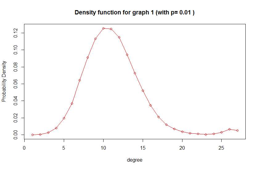
####1.生成一个1000个节点的无向随机图,边概率分别是0.01,0.05,0.1:(就是任意两个节点间有边的概率),判断这些图是不是连通图,并求其直径。
1
2
3
4
5
6
7
8
9
10
11
12
13
14
15
16
17
18
19
20
21
22
23
24
25
26
27
28
29
30
31
32
33
34
35
36
library (igraph)
p <- c(0.01 ,0.05 ,0.1 )
sig <- c(1 ,1 ,1 )
col <-c("red" ,"green" ,"blue" )
for (i in 1 :3 ){
for (j in 1 :100 ){
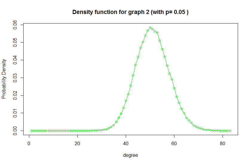
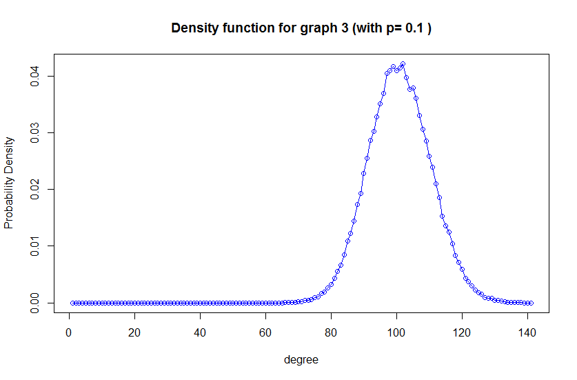
graph<-erdos.renyi.game(1000 ,p[i])
if (sig[i]){
d<-degree.distribution(graph)
sig[i] = 0
}else {
d<- d + degree.distribution(graph)
}
}
d = d/100
plot(d, type="o" , col=col[i],main=paste("Density function for graph" ,i,"(with p=" ,p[i],")" ),xlab="degree" ,ylab="Probability Density" )
}
connect_ <- c(0 ,0 ,0 )
diameter_ <- c(0 ,0 ,0 )
for (i in 1 :3 ){
for (j in 1 :100 ){
graph<-erdos.renyi.game(1000 ,p[i])
if (is.connected(graph)){connect_[i]=connect_[i]+1 }
diameter_[i] = diameter_[i]+ diameter(graph)
}
diameter_[i] = diameter_[i]/100
connect_[i] = connect_[i]/100
cat("when p =" , p[i],",it has probability " ,connect_[i],"the network is connected. " )
cat("Diameter for this network: " ,diameter_[i],'\n' )
}
when p = 0.01 ,it has probability  0.93 the network is connected. Diameter for this network:  5.38
when p = 0.05 ,it has probability  1 the network is connected. Diameter for this network:  3
when p = 0.1 ,it has probability  1 the network is connected. Diameter for this network:  3
erdos.renyi.game() 就是这样一个随机构造图的函数,第一个参数是顶点个数,第二个参数可以是一个概率(表示随机两点之间有边的概率)或者是一个整数值,表示总共有多少条边,还有一个默认参数directed = FALSE,如果为TRUE则是有向图。
degree.distribution() 就是求一个图中度的分布函数如上面三幅图可见一般度就集中在N*P那边。
is.connected() 和 diameter() 分别求图是否是连通图,以及图的半径。
对这个做一个延伸,到底什么时候这个网络是不连通的呢?看到当p = 0.01时并不是所有的图都是连通的了,那有没有一个具体的值,使得当P>Pr时,是连通图,P<Pr时是非连通图?
这里我们用代码去夹逼这个值,我们从0.05作为初始值,以0.0001为步长,不断去计算连通性,计算出临界值,重复50次
1
2
3
4
5
6
7
8
9
10
11
12
13
14
15
16
17
p = 0.05
p_c = 0
iter = 0.0001
for (i in 1 :50 ){
while (1 ){
graph<-erdos.renyi.game(1000 ,p)
if (is.connected(graph)){
p = p - iter
}else {
p_c = p_c + p
break
}
}
}
p_c = p_c /50
cat("when p < " ,p_c,"the generated random networks are disconnected, and when p > " ,p_c,"the generated random networks are connected" )
when p < 0.006976 the generated random networks are disconnected, and when p > 0.006976 the generated random networks are connected
那么这个值究竟是不是定的,以及是怎么定下来的?
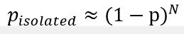
可以参考随机图的维基百科 ,可以看到这个定值其实就是ln(N)/N 所以这里N=1000结果就是 0.00691 和刚刚模拟的 0.006976 很相近,这个ln(N)/N 是如何得来的?
首先孤立点的概率是
然后求孤立点个数的表达式,并令N趋于无穷可以得到
这里在令n=1即可得到P的值为ln(N)/N
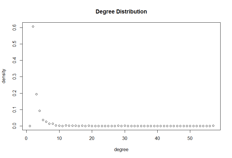
####2.生成一个1000个节点的长尾分布图,判断这些图是不是连通图,并求其直径。
这里我们要使用一个函数 barabasi.game() 这个函数是一个叫 Barabasi-Albert模型的实现,是1999年发表在science上的一篇文章提出的一种随机图生成方法,主要见于电影演员的人际关系网、万维网的网页和美国西部电力节点网等等。有时这种网络又称作无标度网络。服从的是幂律的分布。
成长性 :有别于节点数量固定的方式,BA模型从一张小的网络图开始,逐渐增加节点。
优先连接性 :每当一条新的边被创建,它总是更倾向于连接度数很大的节点,这种 “马太效应”
1
2
3
4
5
6
7
8
9
10
11
12
13
14
15
16
17
18
library ("igraph" )
graph<- barabasi.game(1000 ,directed=FALSE )
d<-degree.distribution(graph)
plot(d, main='Degree Distribution' ,xlab="degree" ,ylab="density" )
connectedness=diameter_=numeric(0 )
for (i in 1 :100 ){
g = barabasi.game(1000 ,directed=FALSE )
connectedness = c(connectedness, is.connected(g))
diameter_ = c(diameter_, diameter(g))
}
Dia_avg = mean(diameter_)
cat("the average diameter of network is" ,Dia_avg,'\n' )
con_avg = mean(connectedness)
cat("it has probability " ,con_avg ,"the network is connected." ,'\n' )
the average diameter of network is 20.11
it has probability  1 the network is connected.
1
2
3
4
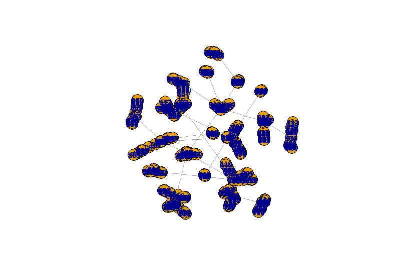
struct = fastgreedy.community(graph)
mod = modularity(struct)
cat("the modularity of this 1000 nodes network is " ,mod,'\n' )
the modularity of this 1000 nodes network is 0.9334264
这里主要看igraph里面的两个函数 fastgreedy.community() 和 modularity() 社区发现 其实社区发现是一个聚类算法,一般有用GN分裂算法划分网络社团。
我们直观地看下由 barabasi.game() 生成的图,可见确实其社区内部边较为密集,而社区之间的边稀疏。